Conferencias sobre computación - Richard P. Feynman
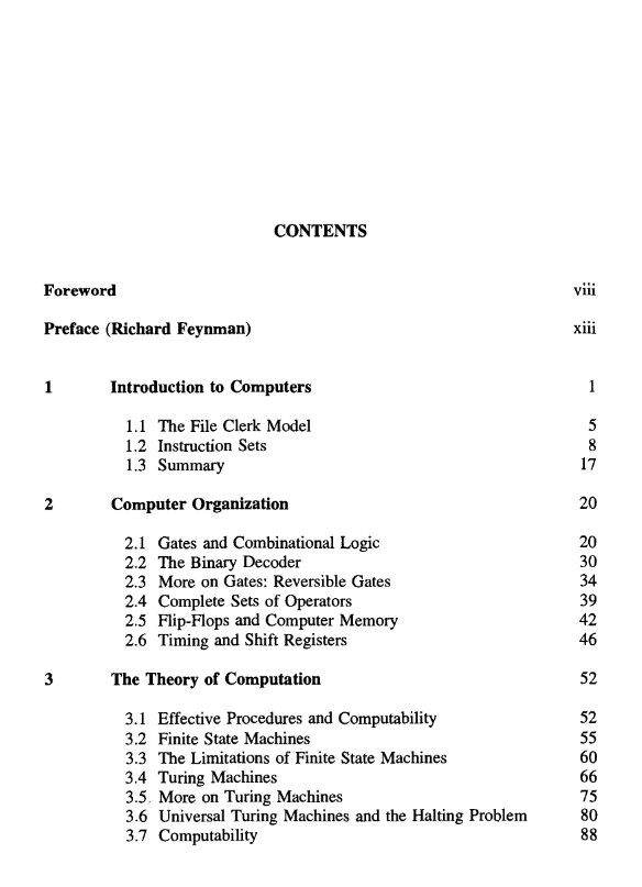
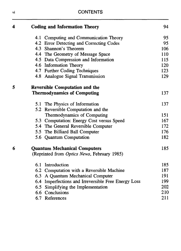
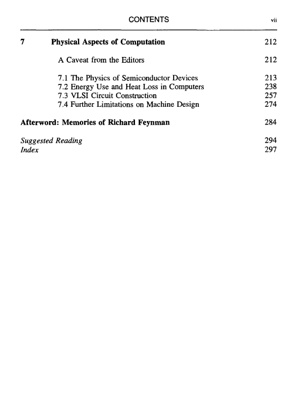
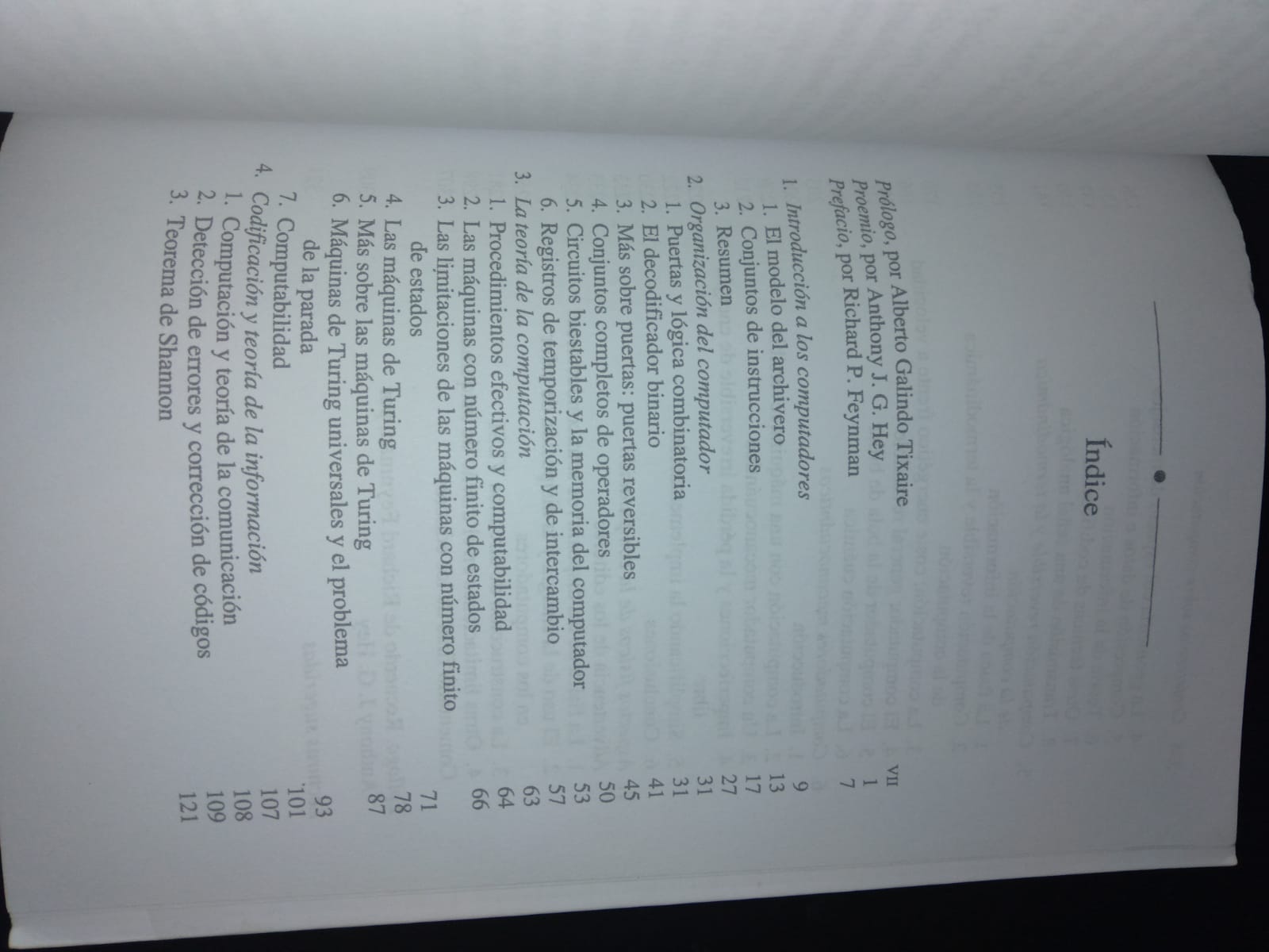
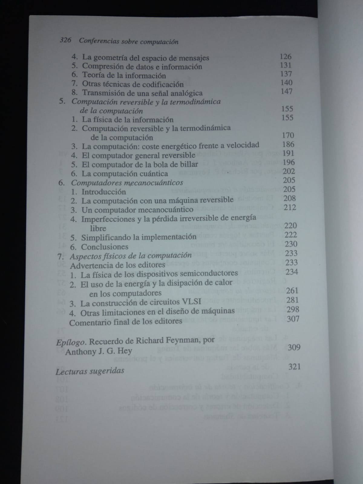
Contents | Índice
Preface | Prefacio

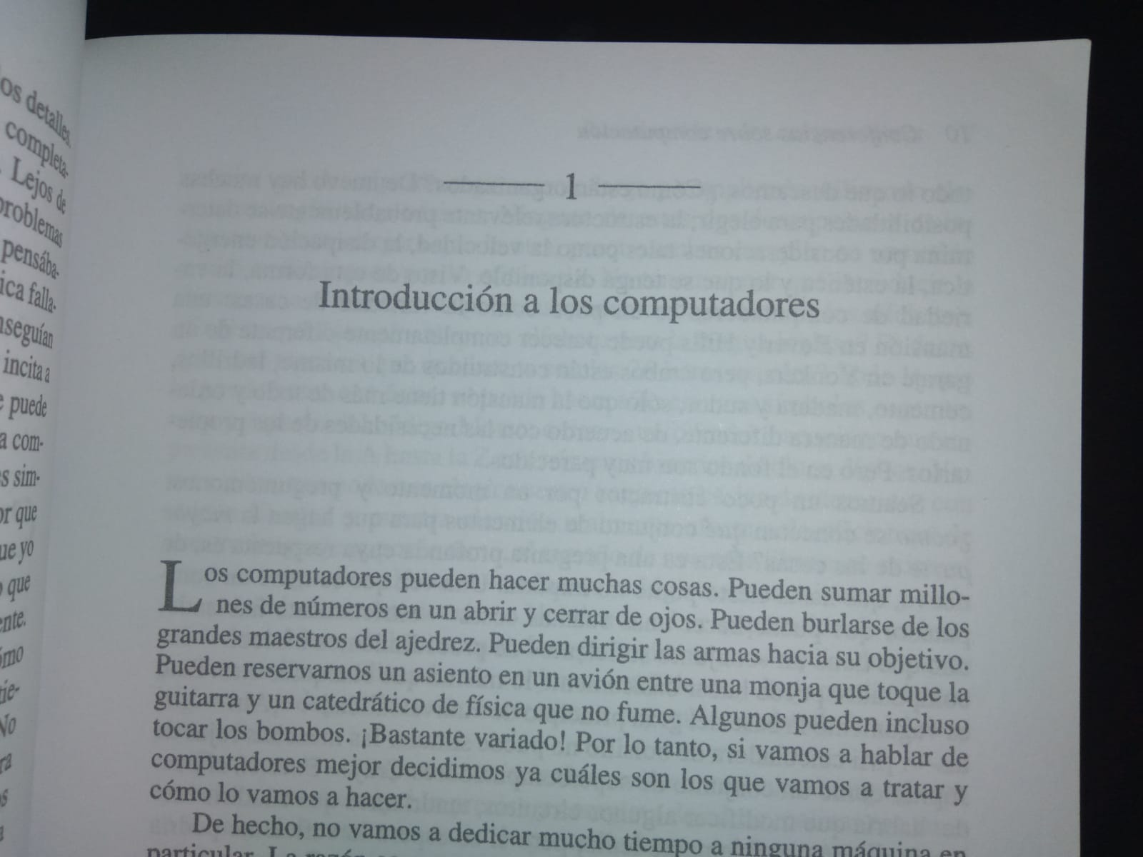
1. Introduction to Computers | Introducción a los computadores

2. Computer Organization | Organización del computador

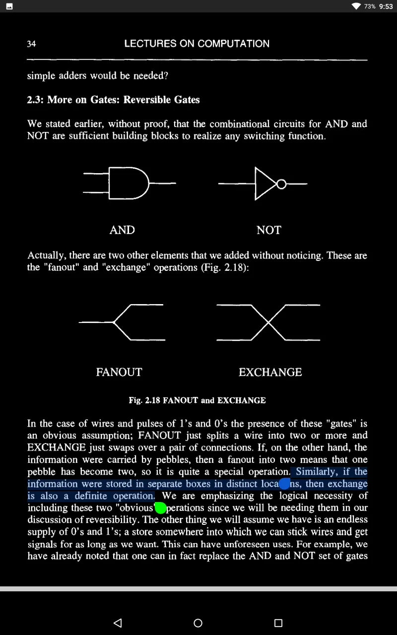
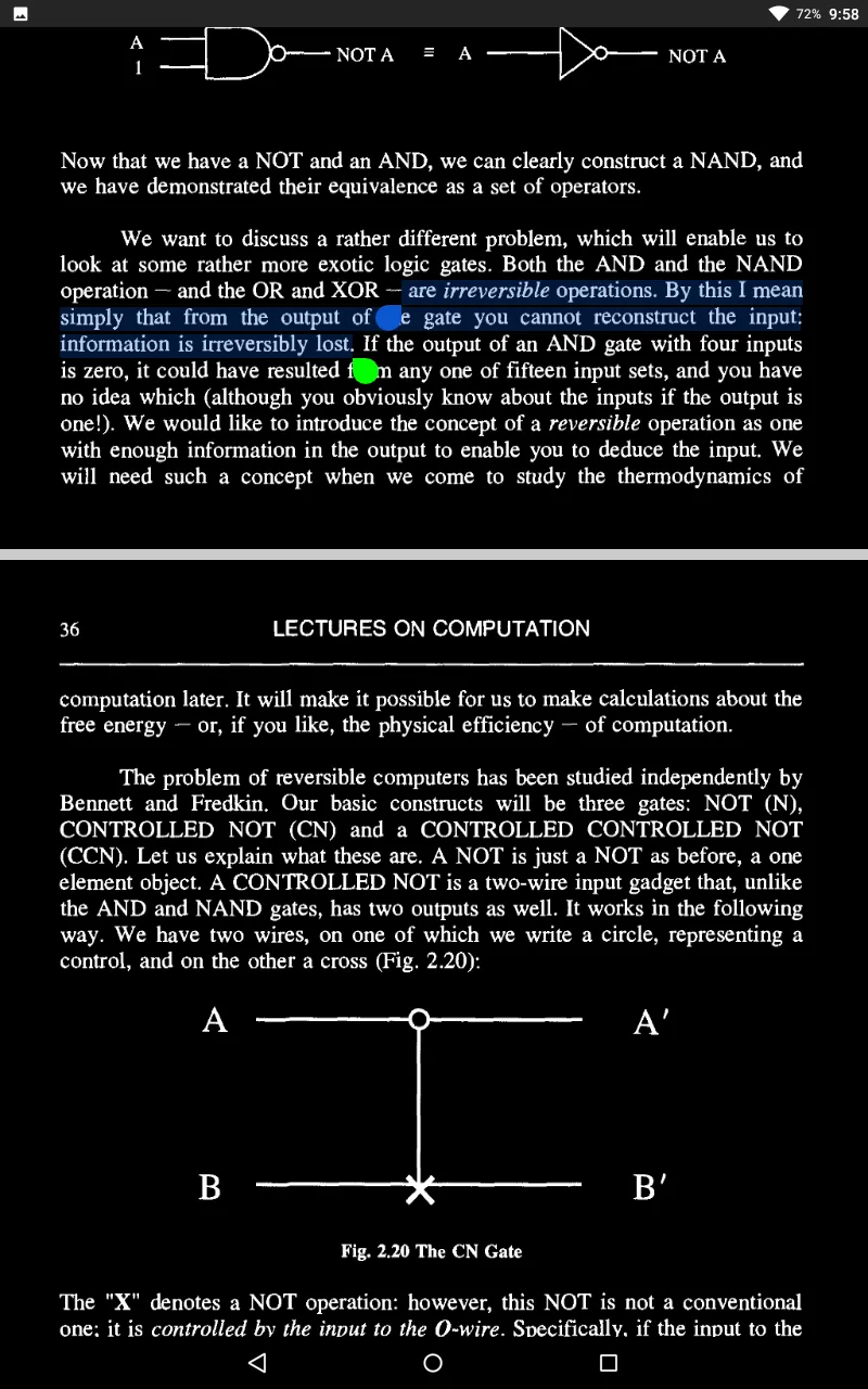
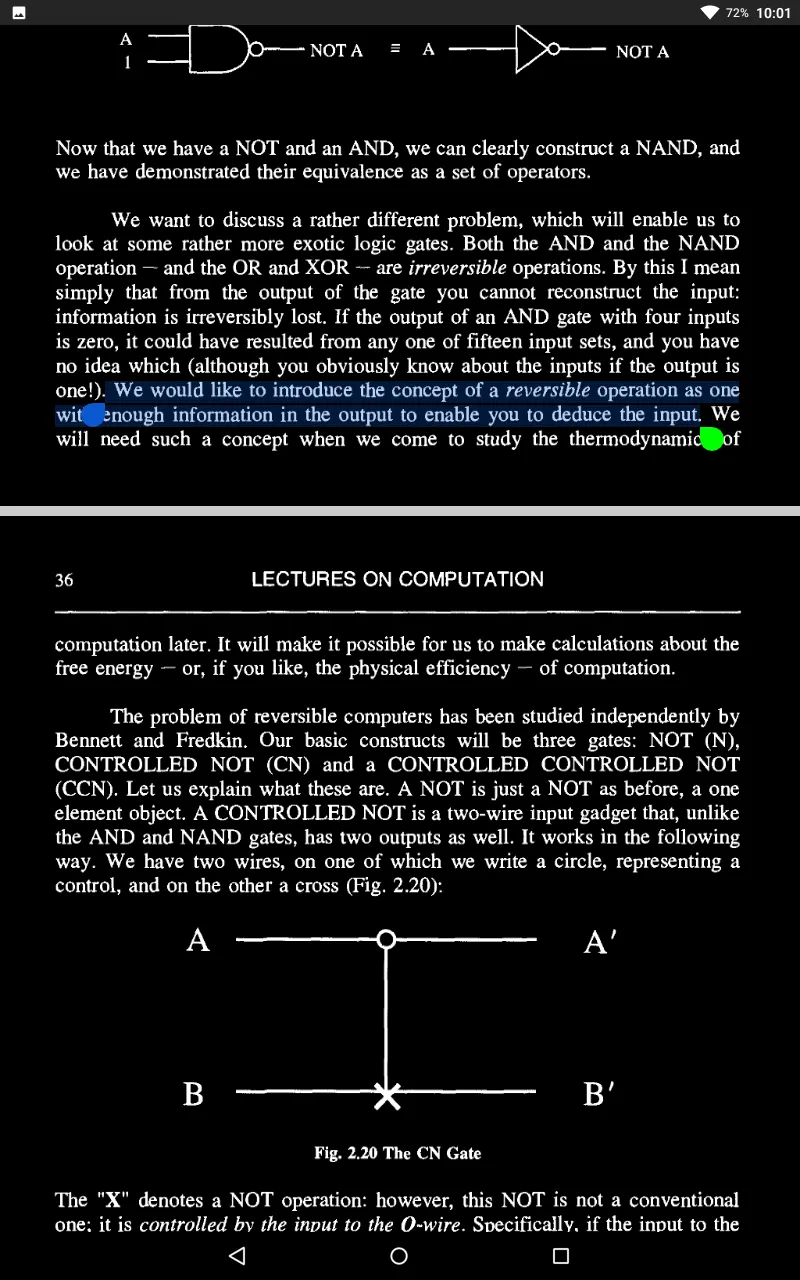
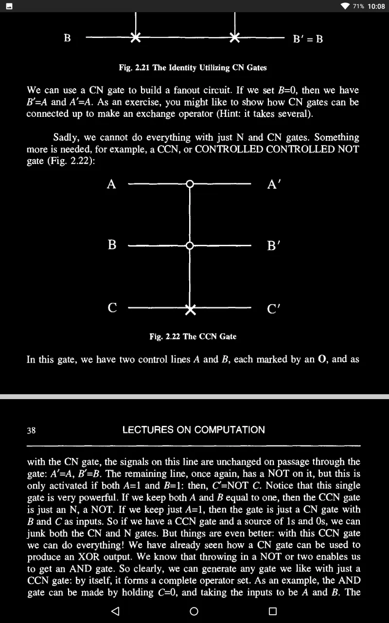
3. The Theory of Computation | La teoría de la computación

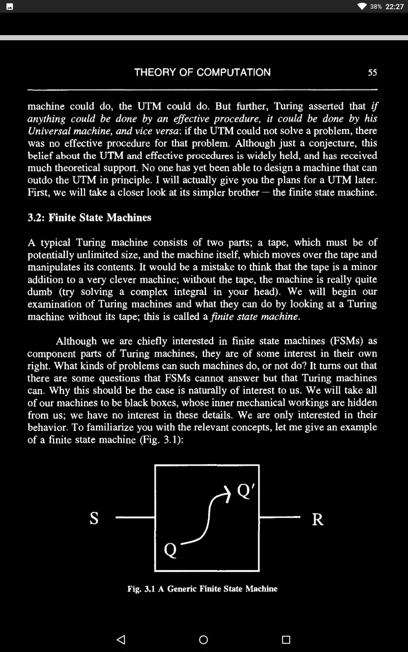
What kinds of problems can such machines do, or not do? It turns out that there are some questions that FSMs cannot answer but that Turing machines can. Why this should be the case is naturally of interest to us.
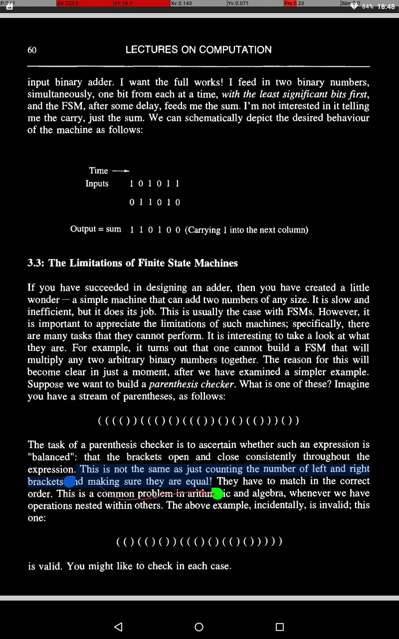
So why cannot an FSM do something this simple?
Here lies the problem. An arbitrary string requires a machine with an arbitrary - that is, ultimately, infinite - number of states. Hence, no finite state machine will do. What will do, as we shall see, is a Turing machine - for a Turing machine is, essentially, an FSM with infinite memory capacity.


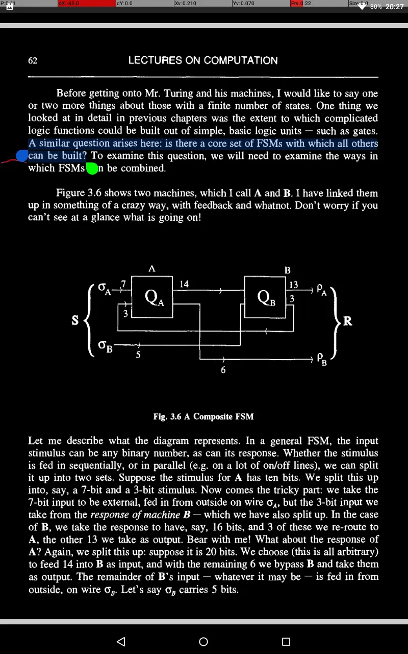
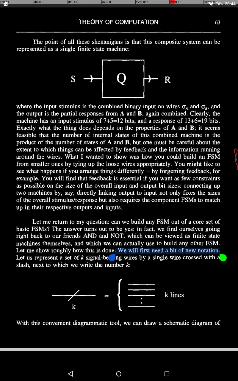

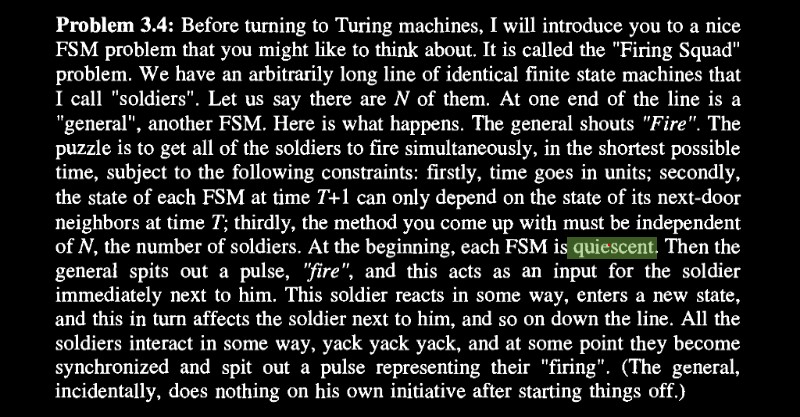

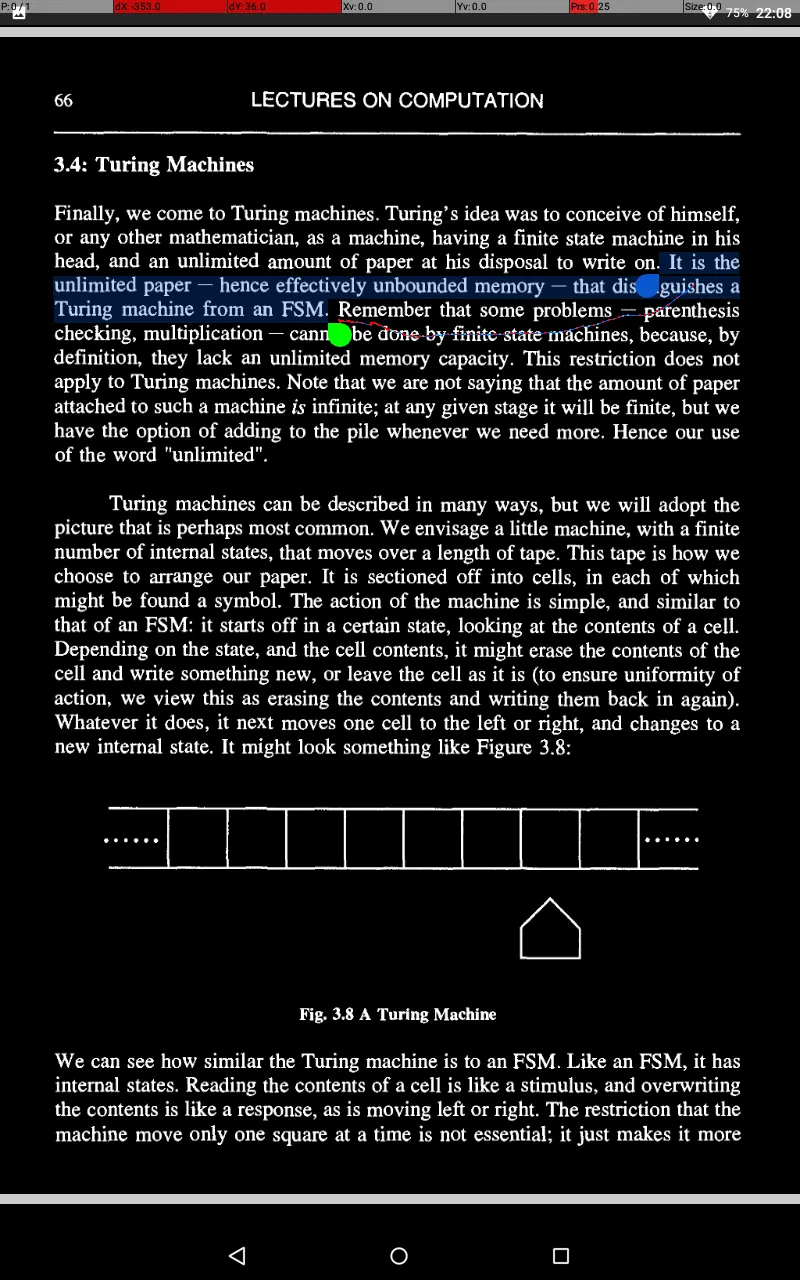


Our discussion closely follows Minsky [1967]. [RPF]
By assigning different symbols to O’s and 1’s - A’s and B’s, say - we can keep track of which were 0’ s and 1’ s; if we wanted to come along tomorrow and use the file again, we could, only we would find it written in a different alphabet.
Minsky’s solution for a locating Turing machine is shown in Figure 3.16:
True to the spirit of Turing machines, we are going to copy it slowly and laboriously to another part of the tape.
A cute feature of this machine is that it copies the contents of the file into the block containing the target filename on the original tape; that is, the target string is overwritten. (We can do this because we chose to have filenames and contents the same size.)
I said earlier that if you had an effective procedure for doing some computation, then that was equivalent to it being possible in principle to find a Turing machine to do the same computation.
the general recursive functions are Turing computable, and vice versa - so we can take “Turing computable” to be an effective synonym for “computable”.
Functions for which this is not true are called “partial”.
This redefined function is complete in the sense that we can assign some numerical value to it for any x.
But in general, we cannot say in advance when a particular value of x is going to give us trouble! Put another way, it is not possible to construct a computable function which predicts whether or not the machine T F halts with input x.
This concept, of Turing machines telling us about other Turing machines, is central to the topic of Universal Turing machines to which we now turn.
Our discussion again closely follows Minsky [1967].
Minsky nicely relates this process to what you would do when using a quintuple list and a tape to figure out what a Turing machine does. The universal Turing machine U is just a slower version of you!
The description of U given above, due to Minsky, requires U to have 8 symbols and 23 states.
surely a machine that can do everything should be enormously complicated? The surprising answer is that it’s not! How efficient one can make a UTM is an entertaining question, but has no deep significance.
In other words, D always halts with an answer. Can such a machine exist? The answer is no! We can actually show that D is an impossible dream,
This is a clear contradiction! Going back through our argument, we find that it is our assumption that D exists that is wrong. So there are some computational problems (e.g. determining whether a UTM will halt) that cannot be solved by any Turing machine. This is Turing’s main result.
Consider computable real numbers: by which we mean those whose binary expansions can be printed on a tape, whether the machine halts or not.
We call a set “countable” if we can put its elements in one-to-one correspondence with elements of the set of positive integers; that is, if we can label each set member by a unique integer.
So by “diagonalization” as it is called (referring to the “diagonal” line we can draw through all of the underlined numbers above) we have shown that the real numbers are not countable. GEB XIII, diagonal de Cantor.
A procedure might take the age of the Universe to complete yet still be technically “effective”. In practice we want procedures that are not just effective but also efficient.
Many problems in “artificial intelligence”, such as face recognition, involve effective procedures that are not efficient - and in some cases, they are not even very effective!
The principle here is that you can know a lot more than you can prove! Unfortunately, it is also possible to think you know a lot more than you actually know. Hence the frequent need for proof.
An effective procedure for this might involve taking all prime numbers up to n l/2 and seeing if any divide n; if not, n is prime.
In mathematics, as in linguistics, a grammar is basically a set of rules for combining the elements of a language, only the language is a mathematical one (such as arithmetic or algebra).
But remember it took a Turing machine to do this: a finite state machine was not up to it.
We will finish our look at computability with an interesting problem discovered by Post as a graduate student in 1921. GEB I, Emil Post.
The question is this: does this process go on forever, stop, or go on periodically? The last I heard, all tested sequences had either stopped or gone into a loop, but that this should be so generally had not been proved.
4. Coding and Information Theory | Codificación y teoría de la información

Components can let us down chiefly in two ways. Firstly, they may contain faults: these can arise during manufacture and are obviously of extreme importance.
What I want to focus on now is a second way in which an element can let us down. This is when it fails randomly, once in a while, perhaps because of the random Brownian motion of atoms or just irregular noise in a circuit.
and the problem of unreliability was acute: with a million components one could expect a thousand of them to be acting up at anyone time!
Indeed, until recently, the problem has ceased to be considered very serious.
Any of these could mean that the message we receive differs from the one sent: this is the so-called “communication problem in the presence of noise”.
Now this isn’t exactly the same situation as with memory - which is like sending a message through time rather than space - but you can see the similarities.
We will start with a look at how we might go about detecting errors, an essential step before we can correct them.
Clearly, all we have to work with is the message: calling up the sender for confirmation defeats the object!
This is an example of coding a message; that is, amending its basic structure in some way to allow for the possibility of error correction (or, of course, for reasons of security).
There are two main shortcomings of this procedure which we should address. Firstly, we might get an error in the parity bit!
Secondly, at best the check only tells us whether an error exists - it does not tell us where that error might be.
Actually, it is a kind of higher- dimensional generalization of the array method.
For any given message, we can ask the question: “How many check bits do I need to not only spot a single error, but also to correct it?” One clever answer to this question was discovered by Hamming, whose basic idea was as follows.
If the syndrome is zero, meaning all parity checks pass, there is no error; if it is non-zero, there is an error, and furthermore the value of the syndrome tells us the precise location of this error.
Each such bit will be a parity check run over a subset of the bits in the full fifteen-bit message.
We assign to each parity check a one if it fails and a zero if it passes, and arrange the resulting bits into a binary number, the syndrome.
Let us look at the rightmost parity check, the far right digit of the syndrome.
To get the second, look at the second digit from the right.
we have narrowed the possible location choices.
We first have to decide where to stick in our parity bits. There is nothing in what we have said so far that tells us whereabouts in the message these must go, and in fact we can put them anywhere. However, certain positions make the encoding easier than others, and we will use one of these.
If we had chosen an apparently more straightforward option, such as placing them all at the left end of the string occupying positions 1 to 4, we would have had to deal with a set of simultaneous equations in a,b,c,d. The important feature of our choice is that the parity positions 1,2,4,8 each appear in only one subset, giving four independent equations.
Note that the cost of these benefits is almost a 50% inefficiency - five check bits for an eleven bit message. As we pointed out earlier however, the inefficiency drops considerably as we increase the message length. For a one-thousand bit message, the inefficiency is a tiny one percent or so.
We can use Poisson’s Law to get a handle on the probabilities of multiple errors occurring when we send our batches.
Now suppose we have no error detection or correction, so we are expending no cash on insurance.
On average, we should only be able to send a thousand batches before this happens, which is pretty miserable.
However, suppose we have our one percent gadget, with single error correction and double error detection. This system will take care of it itself for single errors, and only stop and let me know there is a problem if a double error occurs, once in every million or so batches. It will only fail with a triple error, which turns up in something like every six billion batches. Not a bad rate for a one percent investment!
Issues of efficiency and reliability are understandably central in computer engineering.
Spacecraft communications rely on a kind of voting technique, referred to as “majority logic decisions”.
How many copies you send depends on the expected error rate.
This information is still stored on disks, but individual disks are simply not fast enough to handle the required influx and outflow of data.
Every manufacturer would like to build the perfect disk, one that is error-free - sadly, this is impossible.
The reason you do not usually notice this is that machines are designed to spot flaws and work around them:
However, when a disk is working alongside many others in a parallel processing environment, the momentary hang up as one disk attends to a flaw can screw everything up.
The flaws we are talking about here, in any case, are not really random: they are permanent, fixed on the disk, and hence will turn up in the same place whenever the disk is operating.
The use of this Hamming coding method saved the whole idea of gang disks from going down the drain.
any number will do, but it must be non-zero, or you’ll get into trouble with what follows.

Given this, says Shannon, if no limit is placed on the length of the batches Me, the residual error rate can be made arbitrarily close to zero.
In practice, however, it might require a large batch size; and a lot of ingenuity. However, in his extraordinarily powerful theorem, Shannon has told us we can do it. Unfortunately, he hasn’t told us how to do it. That’s a different matter!
This obviously makes sense. As the error rate drops, the upper limit on the efficiency increases, meaning that we need fewer codebits per data bit.
The actual proof of this theorem is not easy. I would like to first give a hand-waving justification of it which will give you some insight into where it comes from. Later I will follow a geometrical approach, and after that prove it in another way which is completely different and fun, and involves physics, and the definition of a quantity called information.
We now take the logarithm of both sides. The right hand side we work out approximately, using Stirling’s formula:
Taking the Jogarithm to base two of the left hand side of the inequality, and dividing both sides by Me, we end up with Shannon’s inequality.
This inequality tells us that, if we want to code a message M, where the bit error rate is q, so that we can correct k errors, the efficiency of the result cannot exceed the bounds in (4.6).
Now to ask that our error rate be less than a number N (e.g. 10- 3 °) is equivalent to demanding that the number of errors we have to correct be less than K’,
A heck of a lot smaller than our 1O- 30 !

What Shannon has given us is an upper limit on the efficiency.
It’s a terrific mathematical problem.
However, to do this would require a prohibitively long Me, so long that it is not practical. In fact, a scheme is used in which about one hundred and fifty code bits are sent for each data bit!
Message space, simply, is a space made up of the messages that we want to transmit.
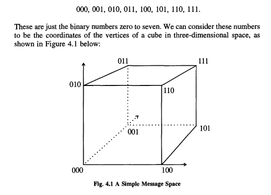
We could easily generalize to a four-bit message, which would have a message space that was a l6-vertex “hypercube”, which unfortunately our brains can’t visualize!
This leads us to introduce a so- called “distance function” on the message space. The one we shall use is called the Hamming distance. The Hamming distance between two points is defined to be the number of bits in which they differ.
The notion of distance is useful for discussing errors. Clearly, a single error moves us from one point in message space to another a Hamming distance of one away; a double error puts us a Hamming distance of two away, and so on.
For a given number of errors e we can draw about each point in our hypercubic message space a “sphere of error”, of radius e, which is such that it encloses all of the other points in message space which could be reached from that point as a result of up to e errors occurring. This gives us a nice geometrical way of thinking about the coding process.
We can build a message space for Me just as we can for M; of course, the space for Me will be bigger, having more dimensions and points. Clearly, not every point within this space can be associated one-on-one with points in the M-space; there is some redundancy. This redundancy is actually central to coding.
Note that we can have simple error detection more cheaply; in this case, we can allow acceptable points in Me to be within e of one another. The demand that points be (2e+ l) apart enables us to either correct e errors or detect 2e.
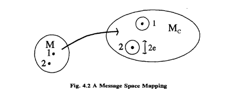
If we wanted single error correction for this system, we would have to use a space for Me of four dimensions.
Using this, we can obtain an inequality relating the volume of Me to that of the spheres.
There is no need to go through the subsequent derivations again; you should be able to see how the proof works out.
You should find that it is actually impossible to detect doubles without bringing in the length of the message.
What the poor parents are doing is converting long English sentences into single bits!
You’re calling long distance but getting the message through costs you nothing because he doesn’t pick up the phone.
SO we could exploit the structure of the language to send fewer symbols, and this packing, or compression, of messages is what we’re going to look at now.
A good way to look at the notion of packing is to ask, if we receive a symbol in a message, how surprised should we be by the next symbol?
What we want to guess is how much freedom we have.
But in any case, people will be able to guess the next letter at a much better rate than one in thirty!
And that gives you an idea of how English can be compacted. It also introduces us to the notion of how much information is in a message.
You cannot get a more efficient sending method than this, compressing a whole message down to one number.
This number, the number of bits we minimally need to send to convey as much as we possibly could have conveyed in the N bits of English (or whatever other system being used) is called the information content, or just the information being sent.
that we are coding messages into a binary system and looking at the bare minimum of bits we need to send to get our messages across.
It is possible to give a crude definition of the “average information per symbol” using the notions we have developed.
In general, of course, the precise answer will be horribly difficult to find.
There can also be “long-range correlations” where parts of the string influence others some distance away. This is true in English, where the presence of a word at one point in a message typically affects what other words can appear near it. As we are not being rigorous yet we will not worry about such problems.
We call this ratio the information per symbol of our system, an interpretation that seems clear from the right hand side of (4.23).
In a sense, the amount of information in a message reflects how much surprise we feel at receiving it.
In this respect, information is as much a property of your own knowledge as anything in the message.
This illustrates how “information” is not simply a physical property of a message: it is a property of the message and your knowledge about it.
In this sense, the string contains a lot of “information”. Receiving the message changes your circumstance from not knowing what it was to now knowing what it is; and the more possible messages you could have received, the more “surprised”, or enlightened, you are when you get a specific one. If you like, the difference between your initial uncertainty and final certainty is very great, and this is what matters.
This makes sense, given our claim that the information in a message represents the “surprise” we experience at receiving it.
This is actually quite an unrealistic assumption for most languages.
Combinatorics comes to our rescue, through a standard formula.
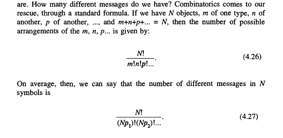
We earlier defined information to be the base two logarithm of the number of possible messages in a string.
That definition was based on the case where all messages were equally likely, but you can see that it is a good definition in the unequal probability case too.
Assuming N to be very large, and using Stirling’s approximation, with which you should be familiar by now, we find:
We can therefore obtain the average information per symbol:
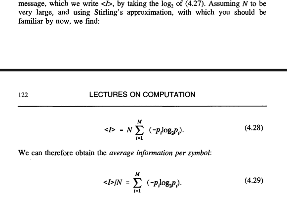
Note how this ties in with our notion of information as “surprise”: the less likely the message to appear, the greater the information it carries.

Incidentally, Shannon called this average information the “entropy”, which some think was a big mistake, as it led many to overemphasize the link between information theory and thermodynamics 6.
This gives the probability Pm of message m being sent and we can treat each message as the symbol of some alphabet, similar to labeling each one, rather like the parent-student card we looked at earlier.
These codes are unlike those we’ve considered so far in that they are designed for messages in which the symbol probabilities vary.
In fact, it is possible to invent a non-uniform code that is much more efficient, as regards the space taken up by a message, than the one we have. This will be an example of compression of a code.
The idea is that the symbols will vary in their lengths, roughly inversely according to their probability of appearance, with the most common being represented by a single symbol, and with the upshot that the typical overall message length is shortened.
Continue in this vein until we reach the right hand of the tree, where we have an “alphabet” of two symbols, the original maximally probable one, plus a summed “joint” symbol, built from all the others.
It is worth pointing out that other Huffman codes can be developed by exploiting the ambiguity that occasionally arises when a joint probability at some point equals one of the original probabilities.
We can easily calculate the length saving of this code in comparison with a straight three-bit code.
It has the property that no code word is the prefix of the beginning of any other code word. A little thought shows that a code for which this is not true is potentially disastrous.
There is an ambiguity due to the fact that the symbols can run into each other. A good, uniquely decodable symbol choice is necessary to avoid this, and Huffman coding is one way forward.
Huffman coding differs from our previous coding methods in that it was developed for compression, not error correction.
However, as I have stressed by the example of English, such dependence is extremely common. The full mathematical treatment of source alphabets comprising varying probabilities of appearance and intersymbol influence is quite complex and I will not address it here. However, I would like to give you some flavor of the issues such influence raises, and I will do this by considering predictive coding.
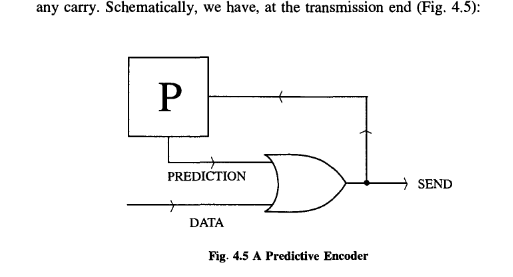
It’s not difficult to see how, if we send this string, we can reconstruct the original message at the other end by using an identical predictor as a decoder. It simply works backwards.
Interspersed between the ones will be long runs of zeroes. The key is this - when sending the message, we do not send these runs: instead we send a number telling us how many zeroes it contained. We do this in binary, of course.
Predictive coding enables us to compress messages to quite a remarkable degree.
You can get pretty close to Shannon’s limit using compression of this sort.
Ordinarily, information like the oil pressure in a car, the torque in a drive shaft, the temperature variation on the Venusian surface, is continuous: the quantities can take any value.
This is not a matter of fundamental principle; it is actually a practical matter. I will say a few words about it despite the fact it is somewhat peripheral. You could say that the whole course is somewhat peripheral.
The secret of sending the value of S is to approximate it.
Then, all we need do is split the interval [0, 1] up into one hundred slices (usually referred to as “bins”), and transmit information about which slice the value of S is in; in other words, a number between 0 and 100.
This is not uncommon. Usually, such a variable will have values that are not evenly distributed.
(very, very few physical quantities have flat probability distributions).
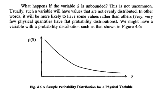
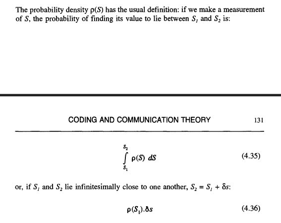
The basic idea for transmitting S in this general case is the same. We divide the effective range of S into a number of bins with the important difference that we size these bins so that they are all of equal probability
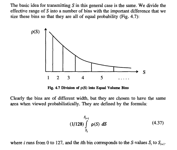
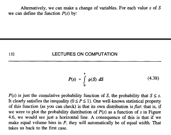
P(s) is just the cumulative probability function of S, the probability that S <= s. It clearly satisfies the inequality (0 <= P <= 1). One well-known statistical property of this function (as you can check) is that its own distribution is flat: that is, if we were to plot the probability distribution of P(s) as a function of s in Figure 4.6, we would see just a horizontal line.
Consideration of such a problem will bring us on to consider the famous Sampling Theorem, another baby of Claude Shannon.
Of course, for a general function, the receiver will have to smooth out the set, to make up for the “gaps”. However, for certain types of continuous function, it is actually possible to sample in such a way as to encode completely the information about the function: that is, to enable the receiver to reconstruct the source function exactly! To understand how it is possible to describe a continuous function with a finite number of numbers, we have to take a quick look at the mathematical subject of Fourier analysis. I will cover this because I think it is interesting;
Recall that, according to Fourier theory, any periodic function f(t) can be written as a sum of trigonometric terms.
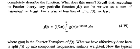
Now the typical function (signal) that is encountered in communication theory has a limited bandwidth;
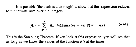
This is the Sampling Theorem.
In other words, if we sampled the function at times spaced (Pi/v) time units apart, we could reconstruct the entire thing from the sample!
Then, the sum (4.41) is no longer infinite and we only need to take a finite number of sample points to enable us to reconstruct f(t).
Although I have skated over the mathematical proof of the Sampling Theorem, it is worth pausing to give you at least some feel for where it comes from.
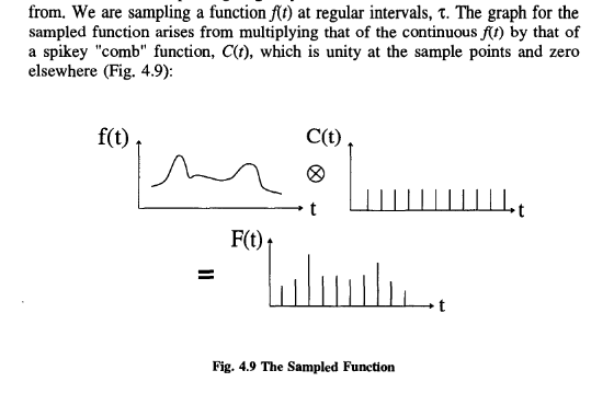
The Fourier transform of the sampled function, F(t), is obtained by the process of “convolution”, which in crude graphical terms involves superposing the graph of <1> with that of X.
There is as much information in one of the Fourier-transformed bumps in Figure 4.11 as there is in the whole of Figure 4.9! As the former transform comes solely from the sampled function F(t), we can see the basic idea of the Sampling Theorem emerging.
Under such circumstances we get what is known as aliasing. The sampling interval will be too coarse to resolve high frequency components inf(t), instead mapping them into low frequency components - their “aliases”.
However, evidence that sampling has occurred often shows up. Maybe the best known is the behavior of wagon wheels in old westerns.
The explanation for this phenomenon lies in inadequate sampling.
To avoid aliasing, we would need to filter out of the signal any unduly high frequencies before we sampled.
Such developments will transform the future.
It seems that the technological world progresses, but real humanistic culture slides in the mud!
5. Reversible Computation and the Thermodynamics of Computing | Computación reversible y la termodinámica de la computación

We want to address the question: how much energy must be used in carrying out a computation?
what is the minimum energy required to carry out a computation?
I am going to illustrate things by concentrating on a particular, very basic physical model of a message being sent.
Since V 2 is smaller than VI’ this quantity is negative, and this is just a result of the convention that work done on a gas, rather than by it, has a minus sign.
We put some in to compress the gas, and conservation of energy says it had to go somewhere.
From the viewpoint of thermodynamics, what we have effected is a “change of state”, from a gas occupying volume V 1 to one occupying volume V 2.
Note that as we are dealing with a finite change here, we have replaced the infinitesimal (gamma) with a finite (delta).
For an irreversible process, the equality is replaced by an inequality, ensuring that the entropy of an isolated system can only remain constant or increase - this is the Second Law of Thermodynamics.
The situation is more fun, too!
What has happened, and this is very subtle, is that my knowledge of the possible locations of the molecule has changed.
and we just average over everything.
Unlike these, it is not a macroscopic property that arises from a sum of microscopic properties. Rather, it is directly related to the probability that the gas be in the configuration in which it is found.
Entropy quantifies this notion.
The gas with molecules going all one way has a W much less than that of the one with a more random - or more disordered - structure, and hence has a lower entropy.
Working isothermally, the momenta of the molecules within the container remains the same (oU=O), but each molecule has access to fewer possible spatial positions.
The fact that the entropy of our compressed gas has dropped is a reminder that the system is not isolated - we have been draining heat into a heat bath.
You can see that if we compress the volume by a factor of 2, then we halve the number of spatial positions, and hence the number of configurations that the molecule can occupy.
We can now return to the topic of information and see where all this weird physics fits in.
Now if the message is a typical one, for some of these bits we will have no prior knowledge, whereas for others we will- either because we know them in advance, or because we can work them out from correlations with earlier bits that we have examined.
Understanding why this is so is worth dwelling on, as it involves a style of argument often seen in the reversible computing world.
Given our assumptions, it is possible to do so, although the downside is that we would have to take an eternity to do it!
Then we must perform a compression, and this will take free energy, as we discussed earlier, as we are lessening our ignorance of the atom’s position.
The net result is zero work to power our machine.
This realization, that it is the erasure of information, and not measurement, that is the source of entropy generation in the computational process, was a major breakthrough in the study of reversible computation.
An interesting question is: How does the occurrence of an error in a message affect its information content?
The first guess, and one that was a common belief for years, was that there was a minimum amount of energy required for each logical step taken by a machine.
The energy required per step is less than kl1ogq, less than kl1og2, in fact less than any other number you might want to set - provided you carry out the computation carefully and slowly enough. Ideally, the computation can actually be done with no minimal loss of energy. Perhaps a good analogy is with friction.
However, physicists are very fond of studying certain types of idealized engines, so-called Carnot heat engines in which heat energy is converted into work and back again, for which it is possible to calculate a certain maximum efficiency of operation.
If your computer is reversible, and I’ll say what I mean by that in a moment, then the energy loss could be made as small as you want, provided you work with care and slowly - as a rule, infinitesimally slowly.
Now you can see why I think of this as an academic subject.
When we come to design the Ultimate Computers of the far future, which might have “transistors” that are atom-sized, we will want to know how the fundamental physical laws will limit us.
In such circumstances, the output carries no more information than the input - if we know the input, we can calculate the output and, moreover, the computation is “reversible”.
The fact that there is no gain in information in our abstract “computation” above is the fIrst clue that maybe there’s no loss of entropy involved in a reversible computation. This is actually correct: reversible computers are rather like Caroot engines, where the reversible ones are the most efficient. It will turn out that the only entropy loss resulting from operating our abstract machine comes in resetting it for its next operation.
We will later show that, in principle, such a calculation can be performed for zero energy cost.
I would now like to take a look in more detail at some reversible computations and demonstrate the absence of a minimum energy requirement.
This seems like a dumb sort of computation, as you’re not getting anywhere, but it is a useful introduction to some of the ideas underlying issues of energy dissipation.
In the second case, clearing the tape will cost free energy, but not for the copy:
Simply, there is no more information in the (data plus copy) set than is in just the single data set. Clearing the system should not, therefore, require more free energy in the first case than the second. This is a common type of argument in the reversible computing world.
The height of the hill, the amount of energy needed for the transition to occur, is called the barrier potential.
To do this, we need to be able to manipulate the potential curve; we have to make the other trough energetically more favorable to the dot.
Furthermore, we assume that the depths of the troughs can be altered by some force of interaction between the copier and the model. (Don’t worry if this is all horribly confusing and abstract! All will become clear.) We’ll call this a “tilt” force, since it tilts the graph.
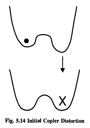
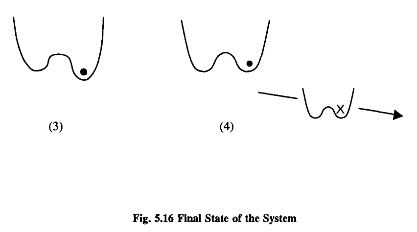
However, if the procedure is graceful enough, the lowering of the barrier, the tilting of the trough and the copying can be done for nothing.
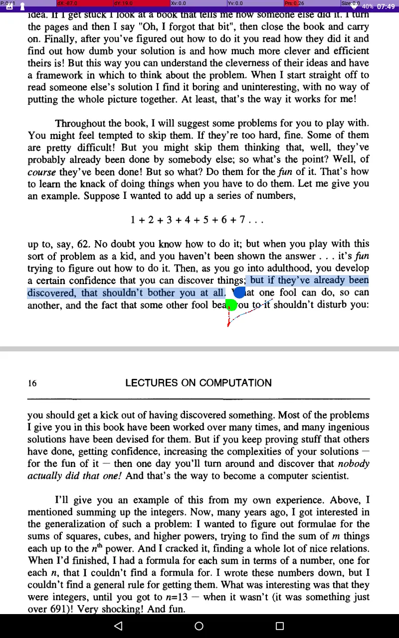
Also it’s nice to work this sort of thing out for yourself: as I said in Chapter One - OK, you’re not the first, but at least you understand it!
The machine that does the copying is an enzyme called RNA polymerase.
In an actual cell, the pyrophosphate concentration is kept low by hydrolysis, ensuring that only the copying process occurs, not its inverse.
Still, 100kT per bit is considerably more efficient than the 10 8 kT thrown away by a typical transistor!
To reiterate: The lesson of this section is that there is no absolute minimum amount of energy required to copy. There is a limit, however, if you want to copy at a certain speed.
It occurs to me that maybe the devices in the machine could all be made reversible, and then we could notice the errors as we go.
That would make this discussion more practical to you and since computing is engineering you might value this! In any case, I shouldn’t make any more apologies for my wild academic interest in the far future.
This will not be a general formula for energy dissipation during computation but it should show you how we go about calculating these things.
The bigger the energy difference E1 - E 2 , the quicker the machine hops from E1 to E 2 , and the faster the computation.
So we can envisage a computer designed so that it proceeds by diffusion, in the sense that it is more likely to move into a state with greater, rather than lower, availability.
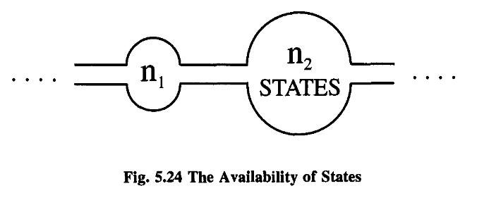
In other words, for this process the energy loss per step is equal to the entropy generated in that step, up to the usual temperature factor.
We can provide a nice physical interpretation of this expression, although at the cost of mathematical inaccuracy.
Generally, then, we will always need a certain amount of junk to remind us of the history of the logical operation.
It is this latter feature that makes reversible computing radically different from ordinary, irreversible computing.
This is your first problem in reversible computing - how to handle subroutines.
The balls all move diagonally across a planar grid and obey the laws of idealized classical mechanics (i.e zero friction and perfectly elastic collisions).
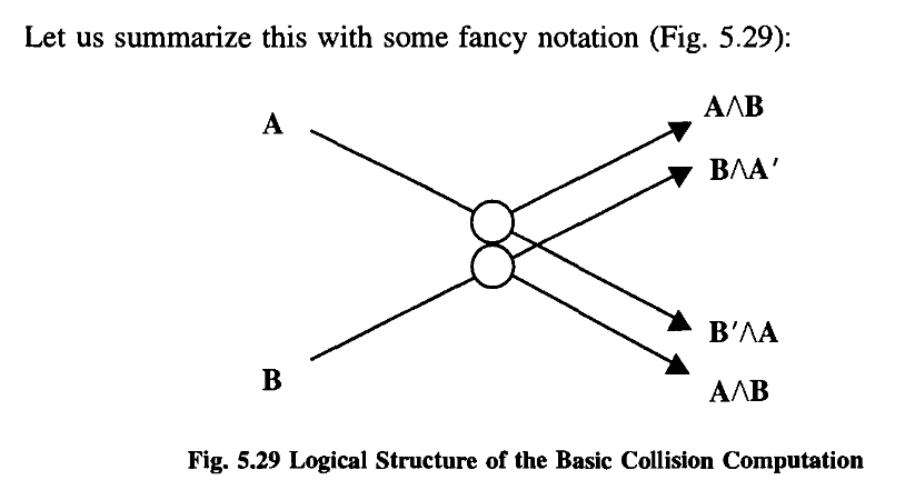
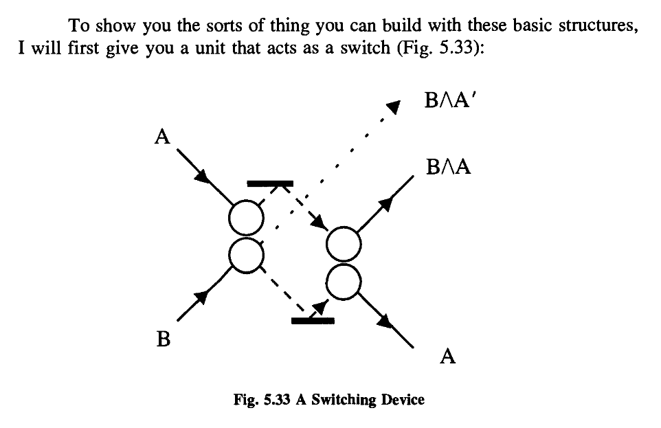
The first, which you would never invent if you were a logician, as it seems a damn silly thing to do, I’ll call a collision gate;
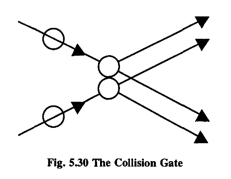
(You might find it an interesting exercise to consider the energy and momentum properties of this gate.)
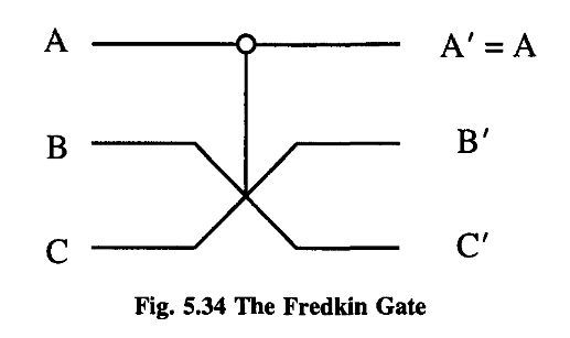
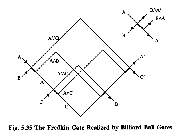
The second and more important device is a redirection gate.

Note that if one ball is missing, the other just sails right through.
In fact, even the tiniest effects of quantum mechanics get in the way. According to the Uncertainty Principle, we cannot know both the precise location and momentum of a ball, so we cannot drop one perfectly straight.
Don’t forget, even your hand will be shaking from Brownian motion!
So how can we claim to have a physically implementable reversible computer?
but we are here discussing questions of principle, not practicality.
(It’ll put some chemists out of a job, but that’s progress).
But the point is that there are no further limitations on size imposed by quantum mechanics, over and above those due to statistical and classical mechanics.
say “up”, which might correspond to an excited state, and “down”, corresponding to a de-excited state.
6. Quantum Mechanical Computers | Computadores mecanocuánticos

We are here considering ideal machines; the effects of small imperfections will be considered later.
Since the laws of quantum physics are reversible in time, we shall have to consider computing engines which obey such reversible laws.
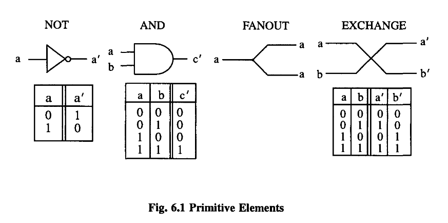
From a logical point of view, we must consider the wire in detail, for in other systems, and our quantum system in particular, we may not have wires as such.
What is the minimum free energy that must be expended to operate an ideal computer made of such primitives?
It could be greatly reduced if energy could be stored in an inductance, or other reactive element.
it seems ridiculous to argue that even this is too high and the minimum is really essentially zero.
What Bennett pointed out was that this former limit was wrong because it is not necessary to use irreversible primitives. Calculations can be done with reversible machines containing only reversible primitives. If this is done, the minimum free energy required is independent of the complexity or number of logical steps i!1 the calculation.
This is a limit only achieved ideally if you compute with a reversible computer at infinitesimal speed.
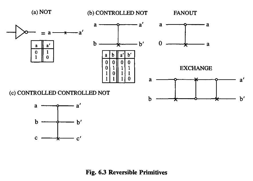
The action is reversed by simply repeating it.
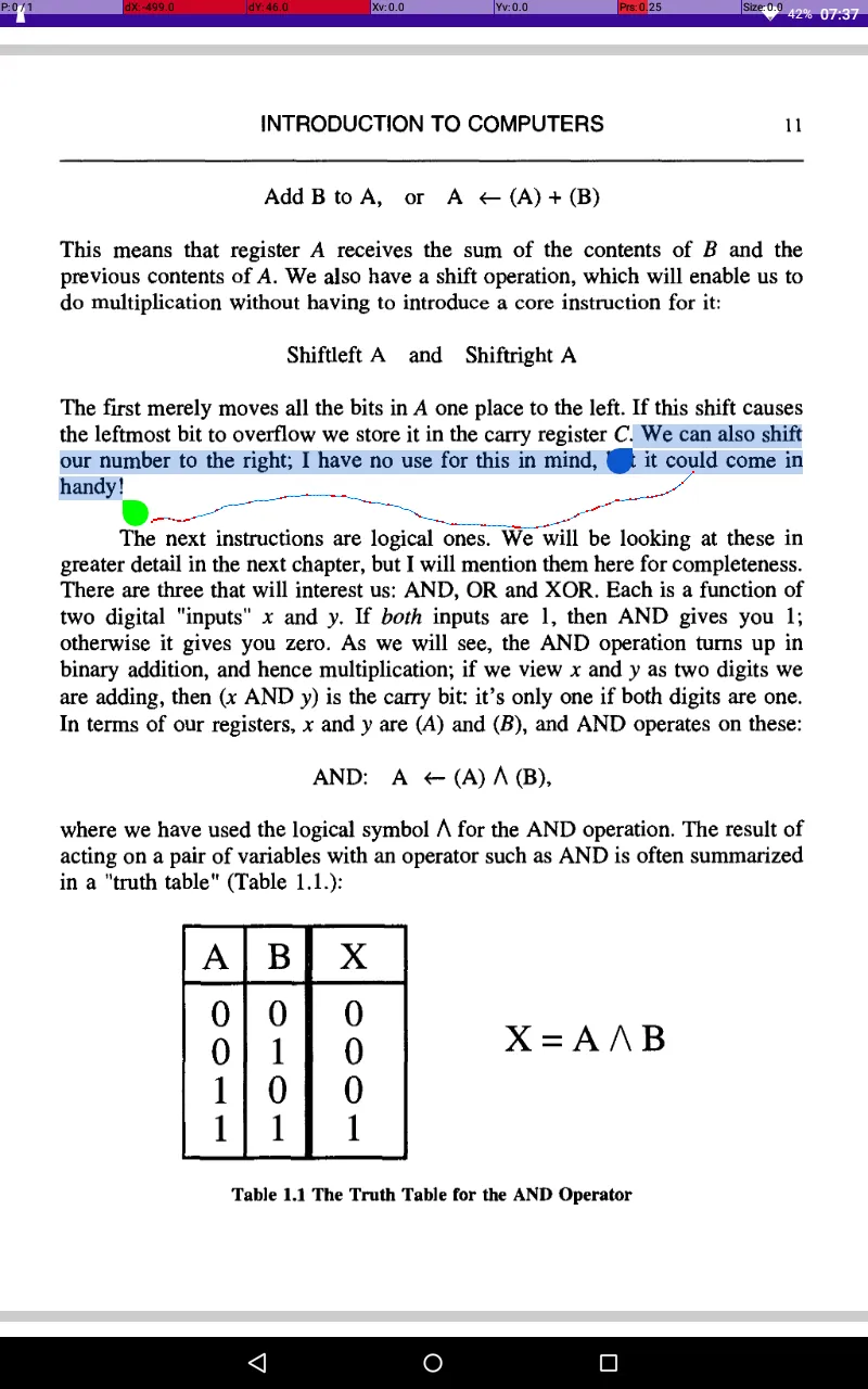
It is likewise the sum modulo two of a and b, and can be used to compare a and b, giving a 1 as a signal that they are different. Please notice that this function XOR is itself not reversible.
The AND function is the carry bit for the sum of a and b.
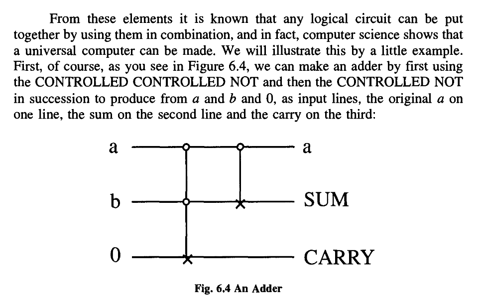
One is the a that we started with, and the other some intermediary quantity that we calculated en route:
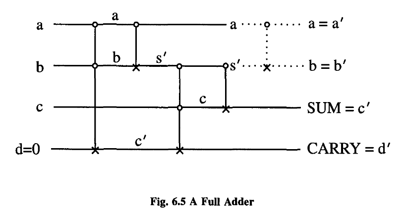
This is typical of these reversible systems; they produce not only what you want in output, but also a certain amount of garbage. In this particular case, and as it turns out in all cases, the garbage can be arranged to be, in fact, just the input.
If the problem you are trying to do is reversible, then there might be no extra garbage, but in general, there are some extra lines needed to store up the information which you would need to reverse the operation. In other words, we can make any function that the conventional system can, plus garbage. The garbage contains the information you need to reverse the process. And how much garbage?
This is reversible because knowing the output and the input permits you, of course, to undo everything. This proposition is always reversible.
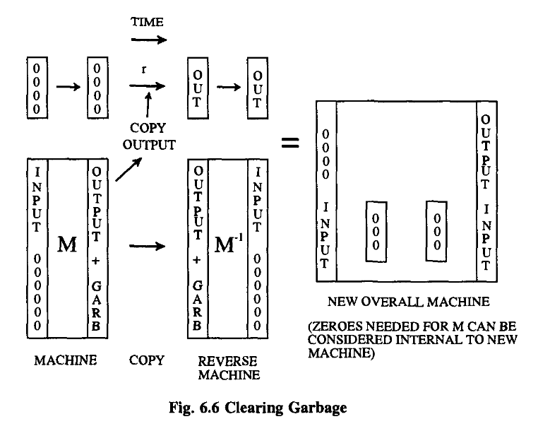
Overall, then, we have accomplished what we set out to do, and therefore garbage need never be any greater than a repetition of the input data.
We are going to write a Hamiltonian, for a system of interacting parts, which will behave in the same way as a large system in serving as a universal computer.
Our Hamiltonian will describe in detail all the internal computing actions but not, of course, those interactions with the exterior involved in entering the input (preparing the initial state) and reading the output.
What we would have then is that the state, in the mathematical form la’,b’,c’> is simply some operation G operating on la,b,c>. In quantum mechanics, state changing operators are linear operators, and so we’ll suppose that G is linear.


It does not matter whether or not the cursor on the j site has arrived there by going directly from 0 to j, or going further and returning, or going back and forth in any pattern whatsoever, as long as it finally arrived at the state j.
In other words, it represents just the waves which are familiar from the propagation of the tight binding electrons or spin waves in one dimension, and are very well known. There are waves that travel up and down the line, and you can have packets of waves and so forth.
Thus the logical unit can act in a ballistic way.
The line is so long that in a real calculation little irregularities would produce a small probability of scattering, and the waves would not travel exactly ballistically but would go back and forth.
What one then could do, would be to pull the cursor along the program line with an external force.
Under these circumstances we can calculate how much energy will be expended by this external force.
That was the entropy lost per scattering.
This is a formula that was first derived by Bennett.
It is very much like a Carnot engine in which, in order to obtain reversibility, one must operate very slowly. For the ideal machine where p is 0, or where you allow an infinite time, the mean energy loss can be O.
The Uncertainty Principle, which usually relates some energy and time uncertainty, is not directly a limitation.
It’s a question of probabilities, and so there is a considerable uncertainty in the time at which a calculation will be done. There is no loss associated with the uncertainty of cursor energy; at least no loss depending on the number of calculational steps.
No further limitations are generated by the quantum nature of the computer per se; nothing that is proportional to the number of computational steps.
In other words, there may be small terms in the Hamiltonian besides the ones we’ve written. Until we propose a complete implementation of this, it is very difficult to analyze.
But until we find a specific implementation for this computer, I do not know how to proceed to analyze these effects.
This computer seems to be very delicate and these imperfections may produce considerable havoc.
The time needed to make a step of calculation depends on the strength or the energy of the interactions in the terms of the Hamiltonian.
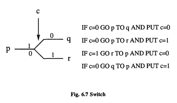
The complex conjugate reverses this.
We shall build all our circuits and choose initial states so that this circumstance will not arise in normal operation, and the ideal ballistic mode will work.
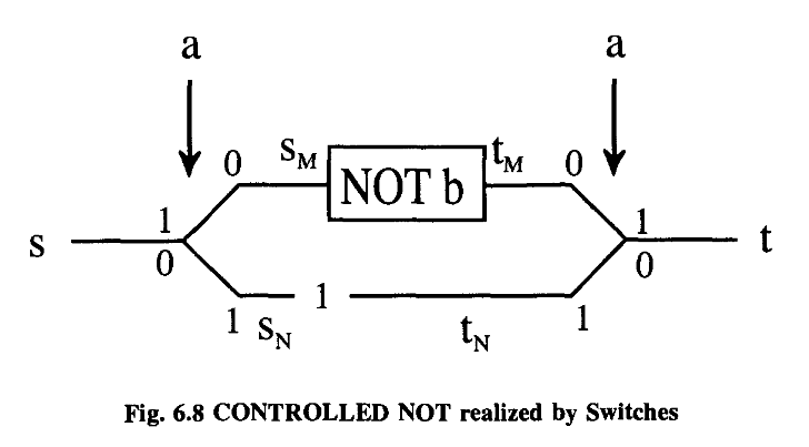
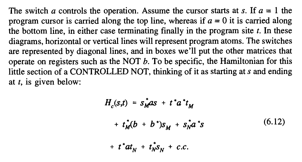
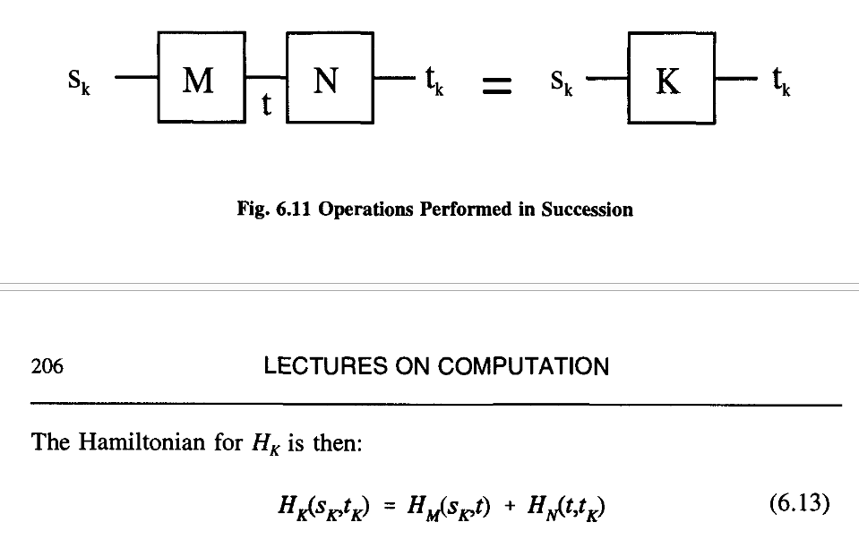
So therefore HM is the part of the Hamiltonian representing all the atoms in the box and their external start and terminator sites.

So between sand t we have a new piece of equipment which has the following properties.
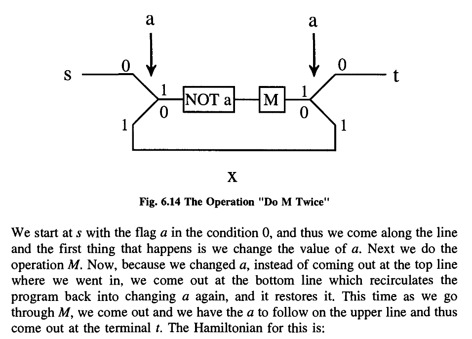
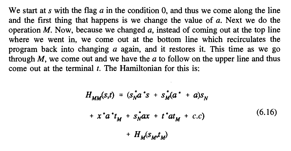
These few examples should be enough to show that indeed we can construct all computer functions with our SWITCH and NOT.
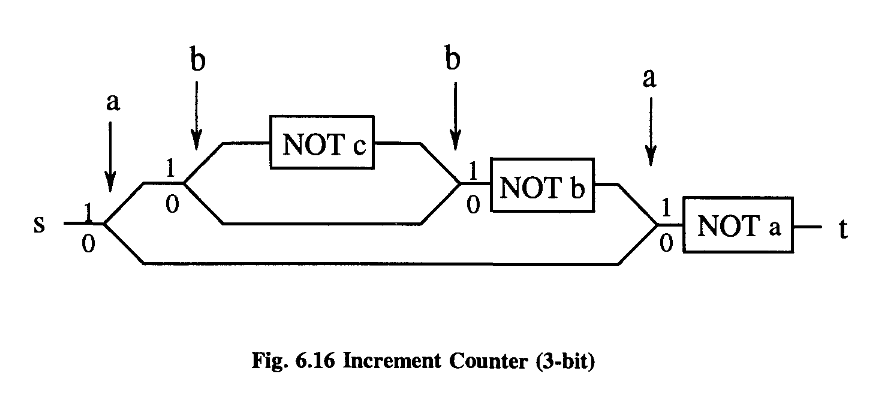
What we have done is only to try to imitate as closely as possible the digital machine of conventional sequential architecture.
What can be done, in these reversible quantum systems, to gain the speed available by concurrent operation has not been studied here.
At any rate, it seems that the laws of physics present no barrier to reducing the size of computers until bits are the size of atoms, and quantum behavior holds dominant sway.
7. Physical Aspects of Computation | Aspectos físicos de la computación

In this way we hope that Feynman’s unique ability to offer valuable physical insight into complex physical processes still comes through.
The unifying theme of this course has been what we can and cannot do with computers, and why.
However, we hope that our presentation will be intelligible to those with only a passing acquaintance with electricity and magnetism,
We shall consider the physical phenomena involved in its operation, and how it works in the engineering context of a Field Effect Transistor.
Our current understanding of the electrical properties of metals and other materials is based on the so-called “Band Theory” of solids.
Typically, there will be a discrete energy gap between the filled and conduction bands. The size of this gap largely determines whether our material is to be classified as a conductor or an insulator, as we’ll see.
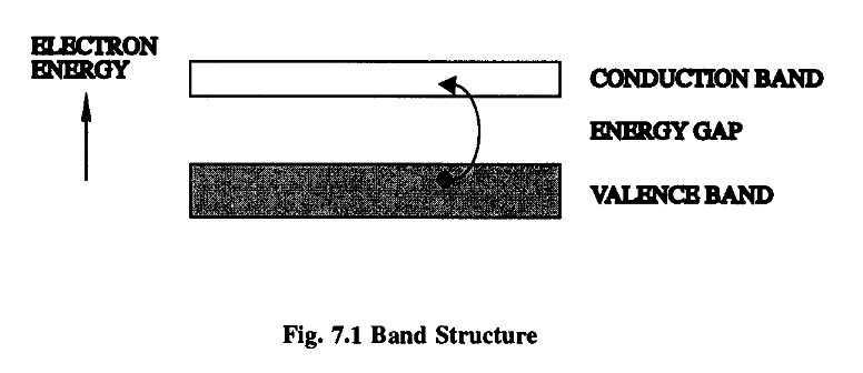
This minimum energy is called the “band gap energy” and its value largely determines the electrical properties of a substance, as I’ve said.
Note that, due to the exponential in the formula, this transition rate rises rapidly with temperature. Nonetheless, for most insulators, this rate remains negligible right up to near the melting point.
This forms the basis of a device called a diode.
The central region is actually depleted of charge carriers and is referred to as the depletion region.
We say that the voltage reverse-biases the junction: in the current flow condition, the junction is said to be forward-biased. We call this device a junction diode and it has the fundamental property that it conducts in one direction but not the other.
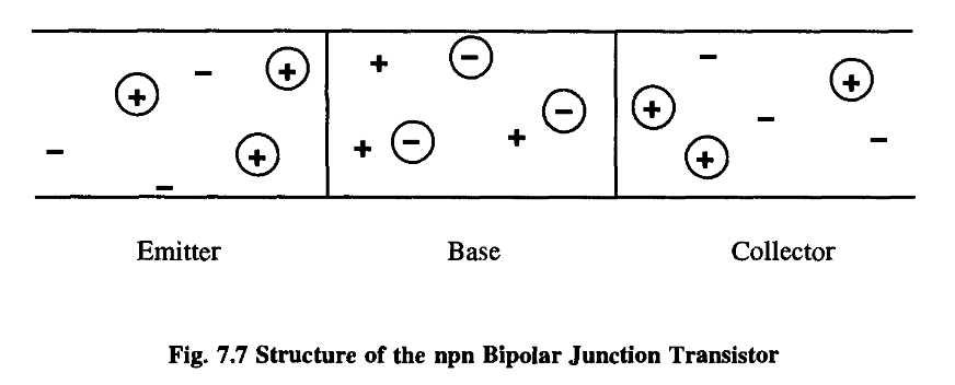
If the doping is of the p-type, we are dealing with so-called nMOS technology; if the substrate is n-type, we have pMOS.
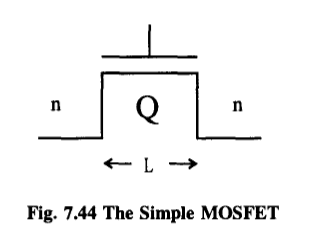
So we have a fantastic device - a switch!
We know that the current Ids is just the charge under the gate divided by the time it takes for the electrons to drift from the source to the drain. This is a standard result in electricity.
we find that the current (charge divided by time) is given by
However, we can see that as long as V ds is fairly small, the transistor has the interesting property that the current through it is proportional to the applied voltage. In other words, it effectively functions as a resistor (remember V = IR!), with the resistance proportional to (1/V gs )’
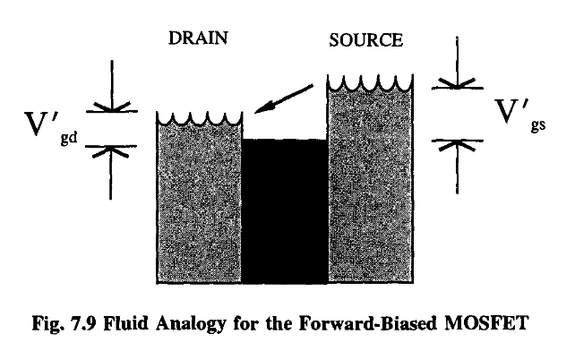
In this situation the transistor is said to be “forward-biased”.
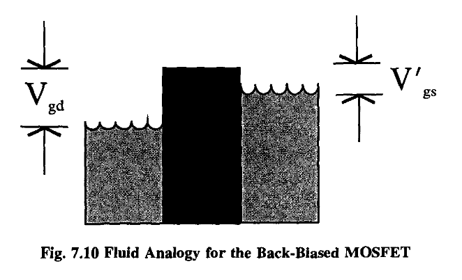
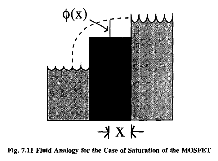
In this instance, where the level of the drain reservoir is below the level of the partition, the water from the source will simply “waterfall” into the drain, at a rate independent of the actual drain-level.
At such a point, the current flow will become constant, irrespective of V ds.
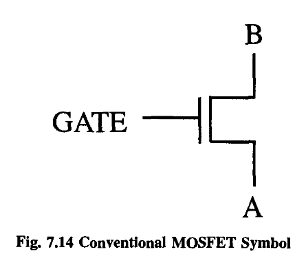
Thus, if we directly connect the source to the gate so that each is automatically at the same voltage, we find our transistor acting no longer as a switch but as a resistance
Now you can see by comparison with the standard formula defining capacitance, Q = CV, that the capacitance of this system displays an extremely non-linear relationship with the plate voltage, V.
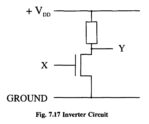
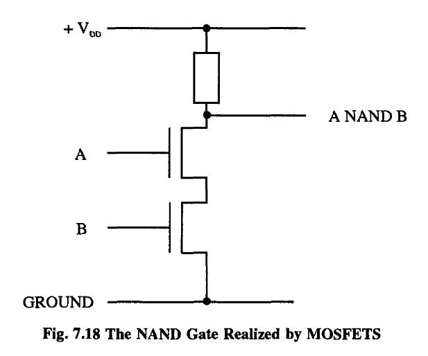
Now there is another essential property of MOSFETs that is not evident from strictly logical considerations. This is their behavior as amplifiers.
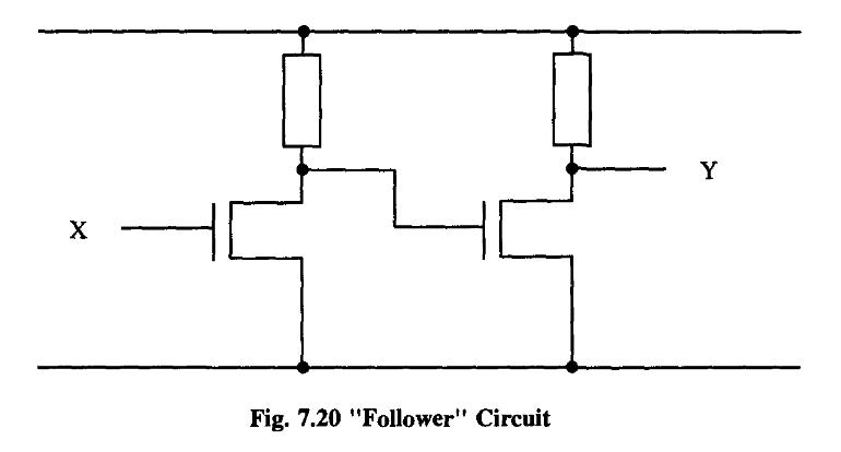
From a logical viewpoint, this is a pretty trivial operation - we have just produced the identity. We’re not doing any computing.
This would indeed be disastrous!
In other words, the output will always represent a definite logical decision, being relatively insensitive to minor power fluctuations along the chain. This circuit is an extremely effective so-called “follower”, which jacks up the power or impedance behind the line (if you like, it is a double amplifier). In a sense, we can control the whole dog just by controlling its tail.
The presence of amplification is essential for any computing technology.
If we can find how long the process takes, and maybe think up ways of speeding it up, we might be able to get better machines.
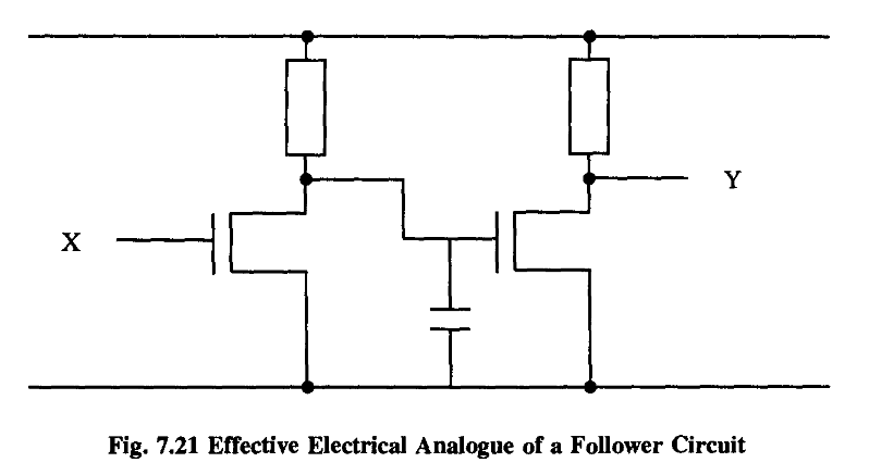
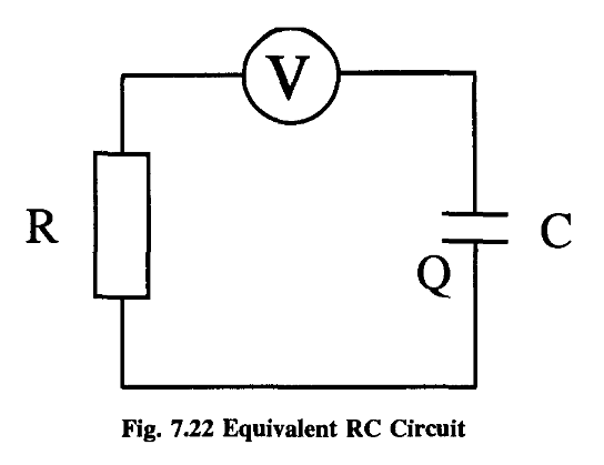

This is a nice example of how Nature places limitations on our technology!
A detailed analysis concluded that propeller-based machines would not work for speeds in excess of that of sound: there was a “sound barrier”.
So even if our transistors aren’t doing anything, they’re throwing away power!
In the CMOS approach, we employ a mixture of n-type and p-type MOSFETs in our circuitry.
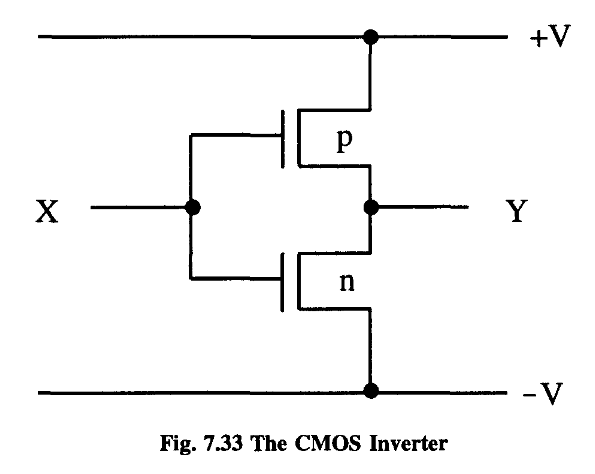
Note that the nMOS depletion mode transistor has effectively been replaced by a conventional p-channel transistor.
The route to - V is cut off by the insulating n-type MOSFET. (I’ll leave it to the reader to see what happens when the input is switched back again.)
This is a remarkable property. In a CMOS inverter, no energy is required to hold a state, just to change it 5 .
The matter of how much energy is required for a logical process was considered in the abstract in Chapter Five, but it is obviously important to get a handle on the practicalities of the matter.
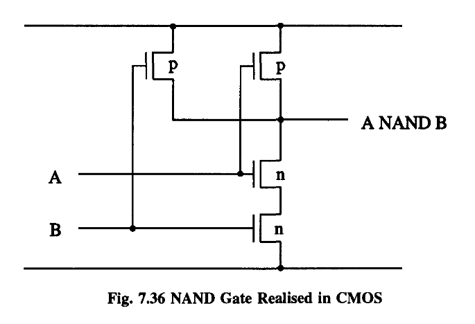
Let’s start by considering in more detail the electrical behavior of a CMOS inverter as part of a chain. This will enable us to examine also the amplification properties of CMOS devices.
The output voltage is an extremely sensitive function of the input since small input changes are magnified many times at the output.
(Remember our analysis in Chapter Five where we saw that kllog2 was theoretically attainable.)
So we have done the stupid thing of getting from one energy condition to the same energy condition by dumping all the juice out of the circuit into the sewer, and then recharging from the power supply!
We start off at sixty miles an hour, and we end up there, but we dissipate an awful lot of energy in the process.
One suggestion is to store the energy in an inductance, the electrical analogue of inertia.
In the process there is noise, friction, turbulence and whatnot, and energy is dissipated. There is a power loss.
We are back where we started, but we have used up a heck of a lot of energy in getting there!
In this case the pressure would be equalized but this finite time to stability results from the fact that water has inertia.
But now if we want the energy of the water back, we just have to open up the adjoining valve to the adjoining tank when the right-hand tank is at a low ebb.
To implement this in silicon we need the electrical analogue of this and that means we need the analogue of inertia. As I’ve said, for electricity this is inductance.
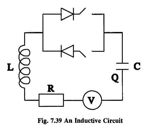
However, that need not mean we have to abandon the basic idea
If we do that, we will unavoidably lose energy.
There is an analogous principle in electricity: Never open or close a switch when there’s a voltage across it. But that’s exactly what we’ve been doing!
In actual circuits, the clocks are much slower than the transistors (e.g., a factor of fifty to one), and so clocking enables us to save a great deal of energy in our computations.

Perhaps we could define two states, in phase with the power supply (logical one) and out of phase (logical zero).
One of the central discoveries of the previous section, which might be general, is that the energy needed to do the switching, multiplied by the time used for this switching, is a constant - at least for resistive systems. We will call this constant the “dissipated action” (a new phrase I just made up).
Does it have to be so tiny? Well, yes, if we want to go as fast as possible.
- you can’t have everything changing too quickly, or you’ll get a jam.
We want to know this to see if, by redesigning such devices, we can get it down a bit, and perhaps use less energy or less time.
Maybe it will help us to understand what is going on here if we define the product of these terms to itself be a dissipated action - just that dissipated during a single collision. This isn’t forced on us: we’ll just see what happens.
Now this is an awful amount, and we would certainly hope that we can improve things somehow!
Firstly, is it completely silly to put things in parallel? Not at all: it’s good for accuracy.
Putting such parts in parallel and deciding the output on the basis of averaging, or by a majority vote, improves system reliability.
And what about putting parts in series? Well, I’ve thought a lot about this, but have yet to come up with any resulting advantage. It wouldn’t help with reliability - all it does is increase the lag. In fact, I can see no reason for having anything other than s = 1.
Current hardware design stinks! The energy loss is huge and there is no physical reason why we shouldn’t be able to get that down at the same time as speeding things up. So go for it - you’re only up against your imagination not Nature.
The (Et) ideas I’ve put forward here are my own way of looking at these things and might be wrong.
How are transistors actually made? How do we, being so big, get all this stuff onto such tiny chips? The answer is: very, very cleverly - although the basic idea is conceptually quite simple. The whole VLSI approach is a triumph of engineering and industrial manufacture, and it’s a pity that ordinary people in the street don’t appreciate how marvelous and beautiful it all is! The accuracy and skill needed to make chips is quite fantastic. People talk about being able to write on the head of a pin as if it is still in the future, but they have no idea of what is possible today!
We do this very cunningly.
We next bombard the wafer with UV light (or X-rays).
The transistor is just the crossing point of a poly silicon path and a diffusion path! Of course, the two paths do not cross in the sense of making physical contact - there is a layer of insulating oxide between them.
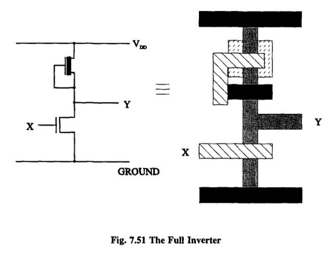
Obviously, some kind of direct contact is needed; otherwise, we would find a capacitor or transistor where the lines cross.
Let us begin by defining a certain unit of length, ‘A., and express all lengths on the chip in terms of this variable.
The metal wire, however, must be at least 3’A. across, to counter the possibility of what is known as “electromigration”, a phenomenon whereby atoms of the metal tend to drift in the direction of the current.
There is a standard heuristic technique for drawing out circuits, one which tells us the topology of the layout, but not its geometry - that is, it tells us what which paths are made of, and what is connected to where; but it does not inform us as to scale, i.e. the relevant lengths of paths and so on.
Since the contents of this memory are to be fixed, we might as well store everything on a Read Only Memory (ROM) device. The only potential hitch in this otherwise straightforward procedure arises from timing: it is conceivable that some instructions could leave the ROM device before the rest, changing the state of the machine and confusing the sensing.
This was how things were done in the early days, carefully building immensely complicated logic circuits, deploying theorems to find the minimum number of gates needed, and so forth, without a ROM in sight.
This output is the set of “what next” instructions corresponding to the particular input.
We now have a device that can manipulate each signal with NOT, AND and OR – in other words, it can represent any logical function whatsoever.
It is a general result that any Boolean function can be factorized in this way.
Incidentally, note, from Figure 7.64 that the generic OR-plane is essentially the AND-plane rotated through a right angle.
This sounds all very straightforward and simple.
Metal, however, has such a low resistance that the load time is relatively much shorter - so if you want to send a signal any great distance, you should put it on metal.
Let it tell us when it’s ready! It carries out its computation, and then sends a signal saying it’s ready to send the data. In this way, the timing is controlled by the computing elements themselves, and not a set of external clocks.
The fact that a decision has to be made introduces the theoretical possibility of a hang-up caused by the data coming in at just such a time that the buffer is not quick enough to make a decision - it can’t make its mind up.
So as we build the machine bigger, the wiring problem becomes more serious.
The problem with this sort of 3-D design, of course, is that for anyone to look at it - to see what’s going on - they have to be able to get inside it, to get a hand or some tools in. At least with two dimensions we can look at our circuits from above!
A natural question to ask is: if we pick a wire at random, what is the chance that is of a certain length? With Rent’s Rule we can actually have a guess at this, after a fashion.
However, if we just deal with orders of magnitude, we shall assume we can neglect this subtlety.
Note that this quantity is divergent:
If we space our cells a little further apart, the size of the machine must balloon out of proportion.
It used to be said in the early eighties that a good designer, with a bit of ingenuity and hard work, could pack a circuit in such a way as to beat Rent’s Rule.
When it comes to the finished product, Rent’s Rule holds sway, even though it can be beaten for specific circuits. Nowadays, we have “machine packing programs”, semi-intelligent software which attempts to take the contents of a machine and arrange things so as to minimize the space it takes up.
These lectures cover interesting topics such as the physics of optical fibers and the possibilities for optical computers.
Moreover, these lectures, by his choice of topics, also demonstrate the subject areas that he felt were important for the fitture.
Afterword: Memories of Richard Feynman | Epílogo: Recuerdo de Richard Feynman

This episode illustrates only a small part of the (healthy) culture shock I experienced in California.
It was only after my wife and I were stopped by the police and asked why we were walking on the streets of Pasadena that I understood the paradox that, in California, you had to have a car to buy a car. Another ‘chicken and egg’ problem arose in connection with ‘ID’ - a term we had not encountered before. As a matter of routine, the police demanded to see our ID and of course the only acceptable ID in deepest Pasadena at that time was a California driver’s license.
I tracked Steve down to the seminar room where I saw he was engaged in a debate with a character who looked mildly reminiscent of the used car salesmen I had recently encountered.
https://dle.rae.es/ethos m. Conjunto de rasgos y modos de comportamiento que conforman el carácter o la identidad de una persona o una comunidad.
Unfortunately for me, my lecture just happened to be a handy vehicle for him to make this point!
There was the obvious distaste of Gell-Mann for the whole approach but that would not have mattered if it had not been for the awkward fact of ‘Feynman’s notebooks’.
Each time Feynman listened, commented and corrected - and then proceeded to derive my ‘new’ results several different ways, pulling in thermodynamics, rotational invariance or what have you, and using all sorts of alternative approaches. He explained to me that once he could derive the same result by a number of different physical approaches he felt more confidence in its correctness. Although this was very educational and stimulating, it was also somewhat dispiriting and frustrating.
I looked at electron-proton scattering when both the electron and proton were ‘polarized’ - with their spins all lined up in the same direction.
Obviously these stories get inflated in the telling but I did ask Feynman about this one since it seemed so out of character to the Feynman I knew.
Certainly he enjoyed making a quick and amusing response.
On one memorable occasion, the speaker started out by writing the title of his talk on the board: “Pomeron Bootstrap”. Feynman shouted out: “Two absurdities” and the room dissolved into laughter.
Feynman could be restrained: on the occasion of another seminar he leaned over to me and whispered “If this guy wasn’t a regular visitor, I would destroy him!”
Feynman credits his “knowing very early on the difference between knowing the name of something and knowing something” to these experiences with his father.
Feynman’ s advice to me on that occasion was: “Y ou read too many novels.” He had started out very narrow and focused and only later in life had his interests broadened out.
and in his unique ability to attack physics problems from many different angles.
For me, it was Feynman’s choice of words that made a Feynman lecture such a unique experience.
In the talk he likened smashing two protons together to smashing two watches together: one could look at the gearwheels and all the other bits and pieces that resulted and try to figure out what was happening.
At a summer school in Erice in Italy one summer he was asked a question about conservation laws. Feynman replied: “If a cat were to disappear in Pasadena and at the same time appear in Erice, that would be an example of global conservation of cats. This is not the way cats are conserved. Cats or charge or baryons are conserved in a much more continuous way.”
Instead, he tells us of all the blind alleys and wrong ideas that he had on the way to his great discoveries.
And, like falling in love with a woman, it is only possible if you do not know too much about her, so you cannot see her faults. The faults will become apparent later, but after the love is strong enough to hold you to her.
Later in the lecture Feynman writes: “1 suddenly realized what a stupid fellow I am; for what I had described and calculated was just ordinary reflected light, not radiation reaction. “
lohannes Kepler - who was first to write down laws of physics as precise, verifiable statements expressed in mathematical terms.
Kepler summed up his struggle with the words: “Ah, what a foolish old bird I have been!”
That was my moment of triumph in which I realized I really had succeeded in working out something worthwhile.”
In the days when calculations like Slotnick’s could take as much as six months, this was the incident that put ‘Feynman’s diagrams’ on the map.
As he says, “learning how to not fool ourselves is, I’m sorry to say, something that we haven’t specifically included in any particular course that I know of. We just hope you’ve caught on by osmosis.” He concludes with one wish for the new graduates: “the good luck to be somewhere where you are free to maintain the kind of integrity I have described, and where you do not feel forced by a need to maintain your position in the organization, or financial support, or so on, to lose your integrity.”
Feynman was never restricted to research in anyone particular field:
It was Feynman’s way of telling the doctor that even in a coma he could hear and think - and that you should always distrust what so-called ‘experts’ tell you!
“He believed in the primacy of doubt, not as a blemish upon on our ability to know but as the essence of knowing. “